Mapping finite element data between non-matching meshes

For finite element simulations you may need to transfer the result field (displacement, temperature, internal variables…) from one mesh to another which is in general different from the previous one. This can happen in particular

• when multiphysics are coupled, for instance in fluid-structure interaction pressure field from the fluid domain needs to be projected onto the solid surface.
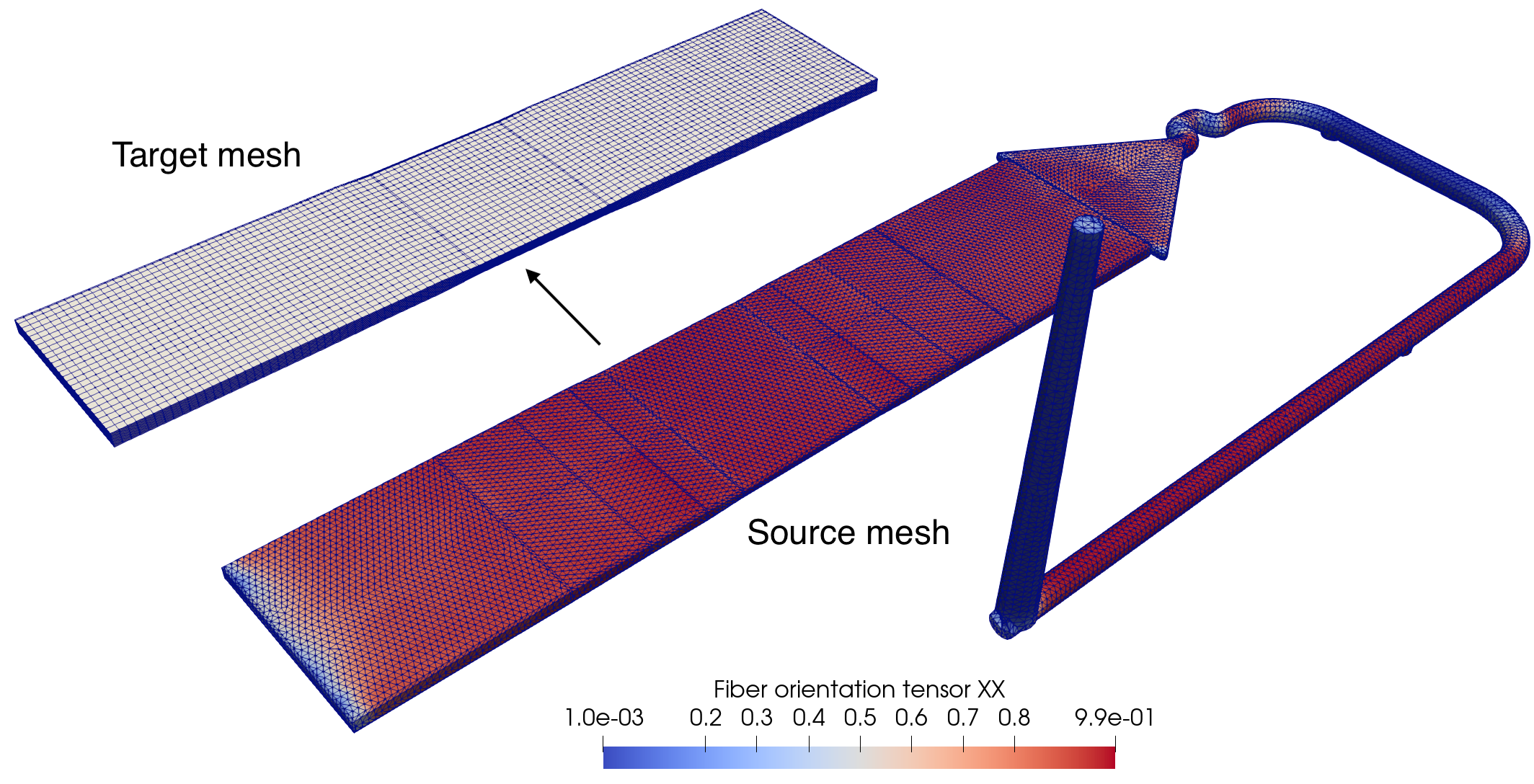
• when multiphysics are chained, in which case the latter simulation is often called an integrative one (i.e. that takes into account previous results). This can happen for example for injection-molded fiber-reinforced plastic parts (during my time in the Promold company), when the fiber orientations (a symmetric tensor defined at nodes) computed by injection molding software (like Autodesk Moldflow or Moldex3D) are transferred to the structural mesh for mechanical simulations. The transferred fiber orientations are then used to compute the anisotropic and heterogeneous mechanical properties of the plastic part. The figure below illustrates an example of such process, where the source mesh (injection molding) is composed of tetrahedral elements and include the additional gate and runners. The target structural mesh, however, is comprised of hexahedral elements and are slightly coarser than the source mesh.
• when remeshing occurred, for adaptive methods or in case of discrete crack propagation.

The field to be transferred can be a scalar, a vector or a tensor, and are discretized using finite elements. It can be defined¹ at the nodes of the source mesh (like \(P_1\) or \(P_2\) fields) or in the cells (\(P_0\) or on Gauss points). Depending on the physics or numerical schemes used, the values of this field can be mapped to the nodes, or into the cells of the target mesh (or elsewhere if you want). This process of transferring finite element data between non-matching meshes is often called mapping, projection or interpolation. The objective of this post is to present a newly developed software interface to this problem using only open-source solutions: MEDCoupling and ParaView.

A bit of theory

Some basic problematics of the mapping theory are recalled here. Interested readers are invited to refer to some research papers on this subject, like Bussetta, P., Boman, R., & Ponthot, J. P. (2015). Efficient 3D data transfer operators based on numerical integration. International Journal for Numerical Methods in Engineering, 102(3-4), 892-929.

The heuristic and most used mapping method consists of the following two steps.

1. Locate each new support point (on which the transferred field is defined in the target mesh: nodes or cell centroids for example) in a particular cell of the source mesh.
2. Perform cell-wise interpolation operations in the source mesh to compute the field value on that new support point.

If the second step is a forward operation only involving evaluations of the shape functions on a particular spatial point, the first step is essentially an inverse operation. In computational geometry terminology, it is referred to as the point location problem for unstructured meshes. Several data structure (trees) can be used to improve computational efficiency of this problem.

When the field to transfer is of a particular physical nature, it is desirable that the mapping operation satisfy the corresponding conservation law. For the density field \(\rho\) for instance, its integral should be preserved before and after mapping to guarantee mass conservation

\[\int_{t}\rho\,\mathrm{d}x=\sum_{s\in\Omega_\mathrm{s}}\int_{s\cap t}\rho\,\mathrm{d}x\,,\quad\forall t\in\Omega_\mathrm{t}\,,\]

where \(\Omega_\mathrm{s}\) and \(\Omega_\mathrm{t}\) are respectively the source and target meshes, \(s\) and \(t\) are their respective elements. We prescribe that the integral of the density field is conserved for each cell of the target mesh. Using these conservation equations, the mapping operator can also be developed.

MEDCoupling

MEDCoupling is a C++ library mainly developed by EDF R&D (French electricity company) and CEA (French Alternative Energies and Atomic Energy Commission) dedicated for the previous mapping problem. It works under major operating systems (Windows, Linux or macOS) and a Python interface is also available through SWIG.

The library supports several mapping methods which include P1P0, P1P1, P0P0 and P0P1, where P1 stands for nodal fields while P0 refers to fields that are constant per cell. The mapping method is also complemented by the physical nature of the field which is either intensive (density or averaged variables like temperature) or extensive (mass or integrated variables). If two meshes do not overlap (some part of the mesh is not covered by another mesh), users must also specify whether the conservation property or the maximum property should be favored.

However, from my point of view, the library has two minor API limitations

1. It only works for the MED(-like) mesh format. As its name suggests, this library is mainly developed for the coupling (data transfer, actually) between MED meshes. Although the MED-file library (interface to MED files) is not a strong dependency, users must construct their own mesh structure as a MEDCouplingUMesh object.
2. For standalone use cases (so without the salome platform), users need to compile on their own the source files provided on the salome website. When only the Python interface is needed, it is an unpleasant burden for Pythoners familiar with pip install, especially when some patches are needed for certain operating systems.

The second issue is now partially solved by my redistribution of the MEDCoupling library as a Python package, available on Github. The compiled binary library files are packed as Python wheels and uploaded to the official package index PyPI. With additional patches to the source files, the medcoupling package is now available under Windows, Linux and macOS for Python 3.6 and 3.7. It can now be installed simply by

pip install medcoupling

For the first issue, based on MEDCoupling I developed a new Python package pymapping that works for all mesh formats readable by the generic mesh input/output library meshio. Nevertheless, users must be somehow familiar with Python programming. For occasional uses, an easy-to-use graphical interface is desired. This motivates the development of a new ParaView plugin also open-sourced on Github.

New ParaView plugin developed using its new Python interface VTKPythonAlgorithmBase

Using this new plugin, mapping can now be easily performed within the ParaView environment, as illustrated by the following video.

As for my previous blog post which bridges meshio and ParaView, this plugin is also developed using the new Python interface VTKPythonAlgorithmBase available since the ParaView 5.6 version. Essentially, the plugin carries out the following operations.

• Convert the source and target meshes (VTK mesh object, actually) already loaded by ParaView to the MEDCouplingUMesh objects for MEDCoupling
• Use MEDCoupling to perform mapping, using the parameters chosen by the user
• Expose the mapped field again as a VTK mesh object which will be rendered by ParaView

In terms of graphical interface, ParaView accompanied by this plugin should be comparable to other commercial software for finite element data mapping. The source and target meshes can be superposed and if needed scaled or translated. The field to transfer can also be post-processed before mapping. In terms of actual data transfer, the mapping algorithms provided by MEDCoupling are derived from rigorous physical properties, and are most of all open-sourced! The mapping capacities for peculiar finite elements can be extended by the experienced users.

1. Knowing that the degrees of freedom of a finite element can be defined everywhere, see Periodic Table of the Finite Elements. ↩